AGROFORESTRY IN SASKATCHEWAN
  • About
    • Shelterbelt Carbon Legacy
    • North American Carbon Program
    • History of Prairie Agroforestry
    • People
  • Shelterbelts
    • Management Support Toolbox
    • Shelterbelt Inventory
    • Shelterbelt Removal
    • Shelterbelt Land Suitability
    • Carbon Stocks
  • FAQ
    • Getting Trees
    • Shelterbelt Planning
    • Planting and Watering
    • Pruning Stems and Branches
    • Weed Control
    • Environmental and Insect Damage
    • Renovation Techniques
  • Research
    • Shelterbelts >
      • Carbon Estimator
      • Factsheets
      • Publications
      • Download Data
    • Afforestation >
      • Afforestation Publications
      • Posters
      • Reports
      • Technical Notes
      • Student Theses
    • Agroforestry
    • Biomass Energy
    • Research Trials
  • Applications
    • HOLOS Model Shelterbelt Component
    • Carbon Management Support Tool
    • Shelterbelt DSS
  • Contact
Written by Dr. Beyhan Amichev (2021)
 
 
Picture

Saskatchewan Shelterbelt Carbon Tool
​
(Belt-CaT)

INSTRUCTIONS:

Belt-CaT tool inputs:


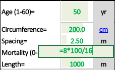
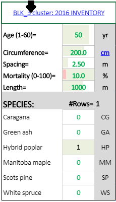
1. Shelterbelt age (years).
  • Enter it in the tool if age is known.
  • Otherwise enter zero (0), then enter the parameters below (items 2-6) - the approximate age of your shelterbelt will be estimated and displayed within the chart.
2. Average tree circumference (cm) over the tree bark is measured at breast height (approximately 1.4 m from ground level) for tree shelterbelts, or at 30 cm height for shrub shelterbelts.
  • This parameter is measured very easily and quickly by wrapping a string around the tree stem (by starting and ending at the same point along the tree stem), and
  • Then measuring with a tape measure the string length between the two points along the string. A demonstration video for measuring tree stem circumference is available here.
  • If multiple stems are present per single tree - measure separately the circumferences for each stem, then enter each value in the circumference tool below. The same approach is used for multi-stem shrubs.
  • Tree stem circumference is used to determine the farm's potential for maximizing shelterbelt ecosystem carbon stocks, calculated as +/- (%), positive/negative potential, relative to a cluster average ecosystem carbon stock in similar shelterbelts. 
3. Spacing (m) is the distance between two neighboring trees within the shelterbelt row.
  • This parameter is also measured very easily and quickly using a tape measure, stretched from the base of one tree to the base of the next tree within the shelterbelt row.
  • For future planned shelterbelts the recommended spacing for deciduous trees (ash, maple, poplar) is 2.5 m (8 ft), for coniferous trees (pine, spruce) is 3.5 m (12 ft), and for shrubs (caragana) is 0.3-1 m (1-3 ft).
4. Mortality (%) is the percent (0-100) of dead trees within the shelterbelt row (if any).
  • This parameter will require a 5-10 min walk along your shelterbelt to count the number of dead tree within a stretch of 25 planted consecutive trees within your shelterbelt row.
  • For example, if you count 8 dead trees (in the 25-planted-trees stretch of your shelterbelt), then mortality (%) is entered in the tool as =8*4, which is 32% mortality (Note: 8*4 = 8*100/25).
  • If there are less than 25 planted trees in your shelterbelt  - for example, if you count 8 dead trees of a total of 16 planted trees in your shelterbelt, then mortality (%) is entered in the tool as =8*100/16, which is 50%.
5. Length (m) is the total length of your shelterbelt.
  • This parameter is determined accurately on your computer.
  • You can trace easily and quickly the total length of your shelterbelt using the web application for the Belt-CaT tool.
6. Species selection and number of rows (#Rows) indicate which species from the list was planted within your shelterbelt and how many rows of trees were planted.
  • If a single species was planted along the entire shelterbelt row - measure and enter the circumference - then enter 1 in #Rows for a single row, 2 for two rows, 10 for ten rows in your shelterbelt, etc. 
  • If multiple species were planted within the same shelterbelt row - enter 0 for circumference - then enter the fraction of each species in the shelterbelt  row. For example, if the row has 15 green ash and 35 caragana that are inter-planted within the same shelterbelt row (15+35=50 plants total), enter =15/50 for green ash (=0.3 fraction) and enter =35/50 for caragana (=0.7 fraction). The Belt-CaT tool will estimate the carbon stocks using the cluster average values.
  • If multiple rows and multiple species were planted in your shelterbelt - enter 0 for circumference - then enter the sum of  fractions for each species estimated from all rows in your shelterbelt. For example: if row-1 has 0.3 green ash and 0.7 caragana, and row-2 has 0.2 Manitoba maple and 0.8 green ash, you should enter 0.7 for caragana, 1.1 for green ash, and 0.2 Manitoba maple. The Belt-CaT tool will estimate the carbon stocks using the cluster average values.
  • For a shelterbelt row planted with a species that is not in the list - measure and enter the circumference - then:
 - For any other Deciduous species (not in the list) - enter 0.5 for  green ash AND 0.5 for Manitoba maple
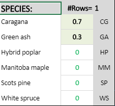
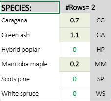
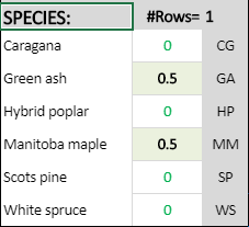
 - For any other Coniferous species (not in the list)- enter 0.5 for Scots pine AND 0.5 for white spruce
 - For any other Shrub species (not in the list) - enter 1 for caragana

7. Shelterbelt design selection and planning - Click on the Top-Left corner of the Belt-CaT tool to access the 2016 INVENTORY of all shelterbelts in your area.
  • The Shelterbelt Inventory Tool (Belt-IT) for your area will be activated in a new window.
  • The Belt-IT tool estimates the C stocks and lengths of all existing shelterbelts in your area which are grouped by a variety of shelterbelt characteristics, such as type, species, condition, width, design, direction, planting length, and age.
  • The output values from the Belt-IT tool provide an evidence-based decision-making for the management and planning of your shelterbelts. 
​

___________________________________________________________________________________________
​
Belt-CaT tool OUTPUTS - chart and table:

How to PRINT your work with the Belt-CaT tool--

1. Click on title of the chart output
2. Then press Ctrl+P (Ctrl and P buttons pressed at the same time) on your keyboard. This will open you printer settings.
3. Adjust your printer settings to print:
  • 1 page per sheet
  • at 70% scale


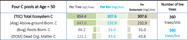
TABLE Outputs - details:

1. (4 C Pools) Carbon stock additions within a planted shelterbelt are reported in 4 C pools as follows:
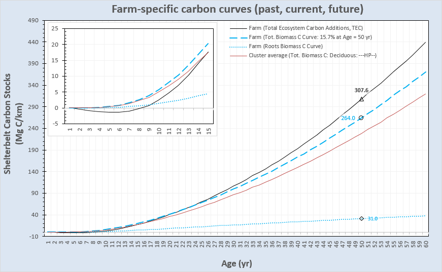
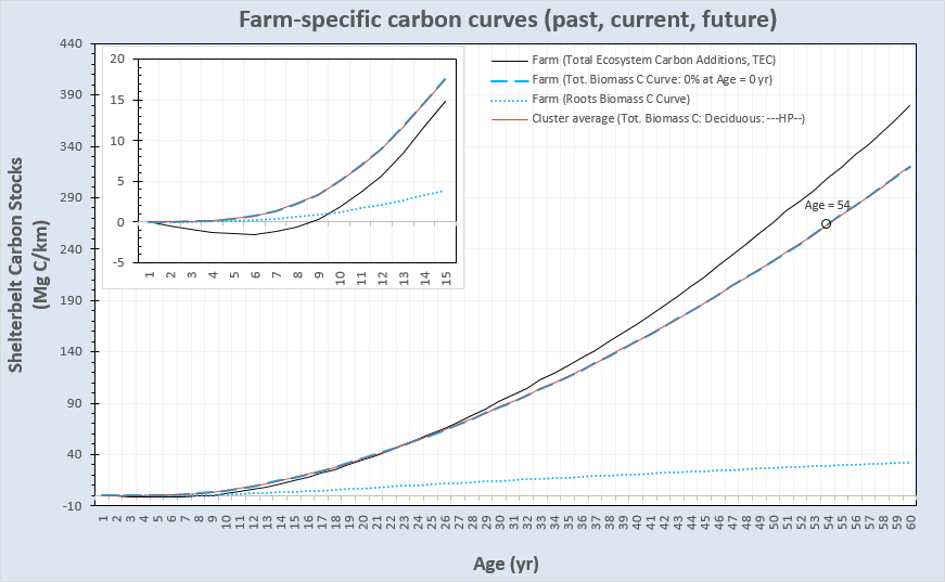
  • (DOM) Dead Organic Matter pool (includes added soil organic carbon, and all dead roots within the soil, dead branches, dead stems, and leaf litter fallen on the soil surface)
  • (Bwg) Below-ground biomass pool (includes all live fine (<10 mm) and coarse roots)
  • (Abg) Above-ground biomass pool (includes all tree/shrub stems, branches, bark, and live foliage)
  • (TEC) Total Ecosystem C pool (includes all three pools, TEC=DOM+Bwg+Abg)
2. (3 C units) Carbon stock additions within a planted shelterbelt are reported in 3 output units:
  • Per tree  - (kg C/tree)
  • Per unit (km) length  - (Mg C/km). This value includes all shelterbelt rows adjusted for 1 km length.
  • Per shelterbelt -  (Mg C/shb). This value includes all shelterbelt rows for the entire shelterbelt length.
3. (Monetary value of C stocks) TEC carbon additions stocks are:
  • Converted to CO2-eq values to estimate a monetary value of the shelterbelt C stocks (based on you market price).
  • Enter a custom market price for 1 tonne of CO2-eq along four ages along the lifespan of your shelterbelt to determine its TEC CO2-eq amount and monetary values.


CHART outputs - details:
​

1. The RED line is the cluster average total biomass C curve (including above-ground and roots biomass C stocks) for the selected species.
  • It is used to estimate your farm's potential to maximize ecosystem carbon stocks in sheltebelts
2. The BLUE dashed-line is the FARM-SPECIFIC total biomass C curve (including above-ground and roots biomass C stocks)
  • It shows past and future trends of carbon stocks accumulation in your sheltebelt.
3. (When age is unknown) The BLACK CIRCLE marks the current status of the shelterbelt
  • It shows AGE on the X-axis, and
  • Total Biomass Carbon (Mg C/km value shown) on the Y-axis.
4. The BLUE dotted-line shows the FARM-SPECIFIC roots biomass C curve.
  • The CURRENT roots biomass C stock (Mg C/km value) is marked by the BLACK DIAMOND.
5. The BLACK line shows the FARM-SPECIFIC Total Ecosystem C (TEC) curve.
  • The CURRENT TEC stock (Mg C/km value) is marked by the BLACK TRIANGLE.


Final note: 

1. If shelterbelt age is unknown (- enter 0 for Age - then enter all other input data)
  • The best approximation of shelterbelt C accumulation (past, current, and future) is the cluster average value for Total Biomass C (RED line) for the selected species.
  • Approximate shelterbelt age will be displayed on the chart, where the RED-line-value is equal to the FARM-SPECIFIC total biomass C value of the shelterbelt (BLACK CIRCLE value).
  • The assumption made is that the average shelterbelt growth for the cluster is representative of the shelterbelt growth on your farm.
2. Planned future shelterbelt carbon stocks: 
 - If your farm has no existing shelterbelts:
  • Enter 0 for Circumference and Mortality
  • Enter 2.5 m for deciduous, 3.5 m for coniferous, or 0.5 m for shrub for Spacing
  • Enter a shelterbelt Age of interest (for example 30 yr). Leave all other default parameters unchanged.
  • All outputs in the table and chart will be estimated for the age using the cluster average values as reference(same species case)
 - If your farm has an existing shelterbelt: 
  • A FARM-SPECIFIC total biomass carbon curve (BLUE dashed-line) is used as reference.
  • Enter all input data for the existing shelterbelt. Modify the number of rows or length if needed.
  • The outputs in the table and chart will apply for the new shelterbelt of the same species - For example, the current growth of an existing hybrid poplar shelterbelt will be a good reference for a future hybrid poplar shelterbelt.
Picture
Picture
Picture
Picture
Picture
Picture
Picture
Picture
Picture
Picture
Picture
Picture
Picture
Picture
 
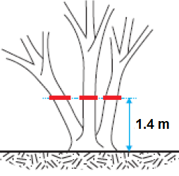
Circumference of multi-stem shelterbelt trees:
Picture
 
Farm potential (%)
1. DEFINITION:
  • Farm potential is estimated from existing shelterbelts as percent increase (positive %) or percent decrease (negative %) of carbon stocks in the farm's shelterbelt, compared to the average shelterbelt carbon stocks for that location (i.e. cluster/soil zone look-up table values).
  • It is estimated as:  Potential (%) = 100 * (C_farm - C_cluster) / (C_cluster)

2. Characteristics - The farm potential represents the cumulative effects on long-term shelterbelt growth of:
  • Soil type (fertility, soil moisture, texture, salinity, pH, etc.)
  • Local weather patterns (wind, rain, snow, temperature, humidity, solar radiation, etc.)
  • Historic shelterbelt maintenance and practices (herbicide, fertilizer, irrigation, tillage, weeding, animal contact/damage, etc.) unique for your farm's conditions
3. Uses - The farm potential percentage is species-specific and applies to all ages of projected shelterbelt growth
  • Future fore-casting - for growth after the year of observation, and
  • Past back-casting - for growth before the year of observation

4. Belt-CaT tool applications:
 - For existing shelterbelts:
  • The farm potential is automatically estimated for any existing shelterbelt using the circumference measurement for the selected species.
  • It is shown in the output window and in the legend of the chart OUTPUT (BLUE dashed line).
  • Positive % - indicates better than cluster average shelterbelt growing conditions. For example:  45%
  • Negative % - indicates worse than cluster average shelterbelt growing conditions. For example:  -45%

 - For future shelterbelts - enter 0 for circumference, then:
  • Enter a new farm potential (%) using an existing shelterbelt (as a reference) on your farm of the same species (see item 4-for existing shelterbelts above), or
  • For a species not found on your farm, leave the default farm potential (%) = 0. This assumes that the cluster average values will be representative of the projected shelterbelt growth on your farm.
Picture

Picture
Copyright © 2018-2030 Centre for Northern Agroforestry and Afforestation. All rights reserved.
​Maintained by Beyhan Amichev
Powered by Create your own unique website with customizable templates.
  • About
    • Shelterbelt Carbon Legacy
    • North American Carbon Program
    • History of Prairie Agroforestry
    • People
  • Shelterbelts
    • Management Support Toolbox
    • Shelterbelt Inventory
    • Shelterbelt Removal
    • Shelterbelt Land Suitability
    • Carbon Stocks
  • FAQ
    • Getting Trees
    • Shelterbelt Planning
    • Planting and Watering
    • Pruning Stems and Branches
    • Weed Control
    • Environmental and Insect Damage
    • Renovation Techniques
  • Research
    • Shelterbelts >
      • Carbon Estimator
      • Factsheets
      • Publications
      • Download Data
    • Afforestation >
      • Afforestation Publications
      • Posters
      • Reports
      • Technical Notes
      • Student Theses
    • Agroforestry
    • Biomass Energy
    • Research Trials
  • Applications
    • HOLOS Model Shelterbelt Component
    • Carbon Management Support Tool
    • Shelterbelt DSS
  • Contact